テスト　STEM教育コードシェア　プラットフォーム

プロンプト
波動関数の指数関数や三角関数の関係が関係をわかりやすく理解するためのコードを出力してください インジケーターを設けてシミュレーションできるようにもできるんでしょうか ちょっと文字が被ってしまっていますねまたは同をどう描くのかもシュミレーションできるようにしてください文字が被らないようにしてください 波動を描く機能も追加してくださいもう一度コードを提供してください よくできました一方で円グラフと波動を一緒に表すことができるはずなのでそのようなコードにしてください先ほどのインジケーターもつけてください

import numpy as np
import matplotlib.pyplot as plt
from matplotlib.widgets import Slider

# --------------------------
# Parameters for the wave function
# --------------------------
k = 2 * np.pi / 5.0         # 波数 (波長 5 単位の場合)
omega = 2 * np.pi / 2.0       # 角振動数 (周期 2 単位の場合)
x = np.linspace(0, 10, 1000)  # 空間座標の配列

# --------------------------
# Figure and Subplots Setup
# --------------------------
fig, (ax_circle, ax_wave) = plt.subplots(1, 2, figsize=(14, 6))
plt.subplots_adjust(bottom=0.3)  # スライダー用のスペース確保

# ----- 左側：単位円（複素平面上の位相ベクトル） -----
theta = np.linspace(0, 2 * np.pi, 500)
ax_circle.plot(np.cos(theta), np.sin(theta), 'k-', lw=1, label='Unit Circle')
ax_circle.set_aspect('equal')
ax_circle.set_xlim([-1.2, 1.2])
ax_circle.set_ylim([-1.2, 1.2])
ax_circle.set_xlabel('Real')
ax_circle.set_ylabel('Imaginary')
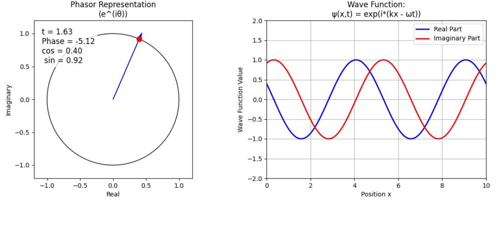
ax_circle.set_title("Phasor Representation\n(e^(iθ))")

# 初期時間 t = 0 における位相は -omega*t = 0
init_t = 0.0
phase = -omega * init_t
# 単位円上の点の描画
point, = ax_circle.plot(np.cos(phase), np.sin(phase), 'ro', markersize=8)
# 原点から点への矢印
arrow = ax_circle.arrow(0, 0, np.cos(phase), np.sin(phase), head_width=0.05, head_length=0.1,
                        fc='blue', ec='blue')
# アノテーション（軸座標で固定表示）
annotation = ax_circle.text(0.05, 0.95, '', transform=ax_circle.transAxes, fontsize=12,
                            verticalalignment='top',
                            bbox=dict(facecolor='white', alpha=0.8, edgecolor='none'))

# ----- 右側：波動関数のプロット -----
# 初期状態: ψ(x,0) = exp(i*(kx)) → 実部 = cos(kx), 虚部 = sin(kx)
line_real, = ax_wave.plot(x, np.cos(k*x - omega*init_t), 'b-', lw=2, label="Real Part")
line_imag, = ax_wave.plot(x, np.sin(k*x - omega*init_t), 'r-', lw=2, label="Imaginary Part")
ax_wave.set_xlim(0, 10)
ax_wave.set_ylim(-2, 2)
ax_wave.set_xlabel("Position x")
ax_wave.set_ylabel("Wave Function Value")
ax_wave.set_title("Wave Function:\nψ(x,t) = exp(i*(kx - ωt))")
ax_wave.legend()
ax_wave.grid(True)

# --------------------------
# Slider の設定（時間 t のインジケーター）
# --------------------------
slider_ax = plt.axes([0.2, 0.1, 0.6, 0.03])
time_slider = Slider(slider_ax, 'Time t', 0, 10, valinit=init_t)

# --------------------------
# 更新関数：スライダーの値が変わるたびに両方のプロットを更新
# --------------------------
def update(val):
    t = time_slider.val
    # 単位円の更新：位相 = -omega*t
    new_phase = -omega * t
    # 点の位置更新
    point.set_data(np.cos(new_phase), np.sin(new_phase))
    # 古い矢印を削除して新しい矢印を描画
    global arrow
    if arrow is not None:
        arrow.remove()
    arrow = ax_circle.arrow(0, 0, np.cos(new_phase), np.sin(new_phase),
                             head_width=0.05, head_length=0.1, fc='blue', ec='blue')
    # アノテーションの更新（固定位置で表示）
    annotation.set_text(f"t = {t:.2f}\nPhase = {new_phase:.2f}\ncos = {np.cos(new_phase):.2f}\n sin = {np.sin(new_phase):.2f}")
    
    # 波動関数の更新：ψ(x,t)=exp(i*(kx-ωt))
    psi = np.exp(1j * (k * x - omega * t))
    line_real.set_ydata(np.real(psi))
    line_imag.set_ydata(np.imag(psi))
    
    fig.canvas.draw_idle()

time_slider.on_changed(update)

plt.show()